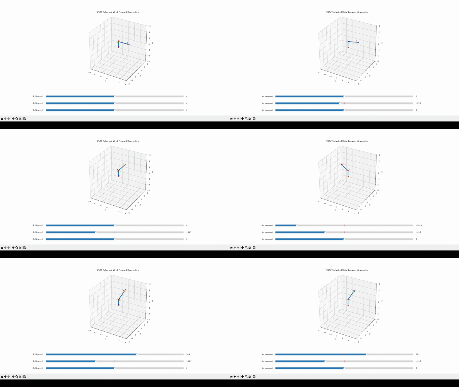
Joint-angle sliders update the DH frames and resulting wrist pose.
Inverse kinematics
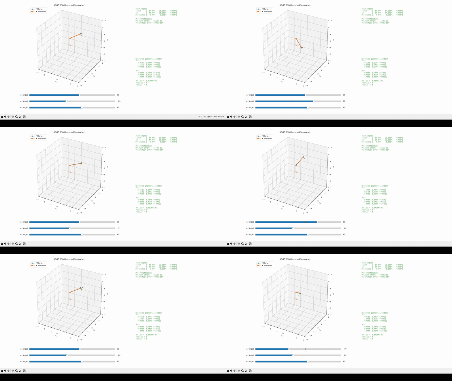
Target and recovered IK poses are compared alongside pose error, Jacobian matrices, determinant, and rank.
Velocity kinematics
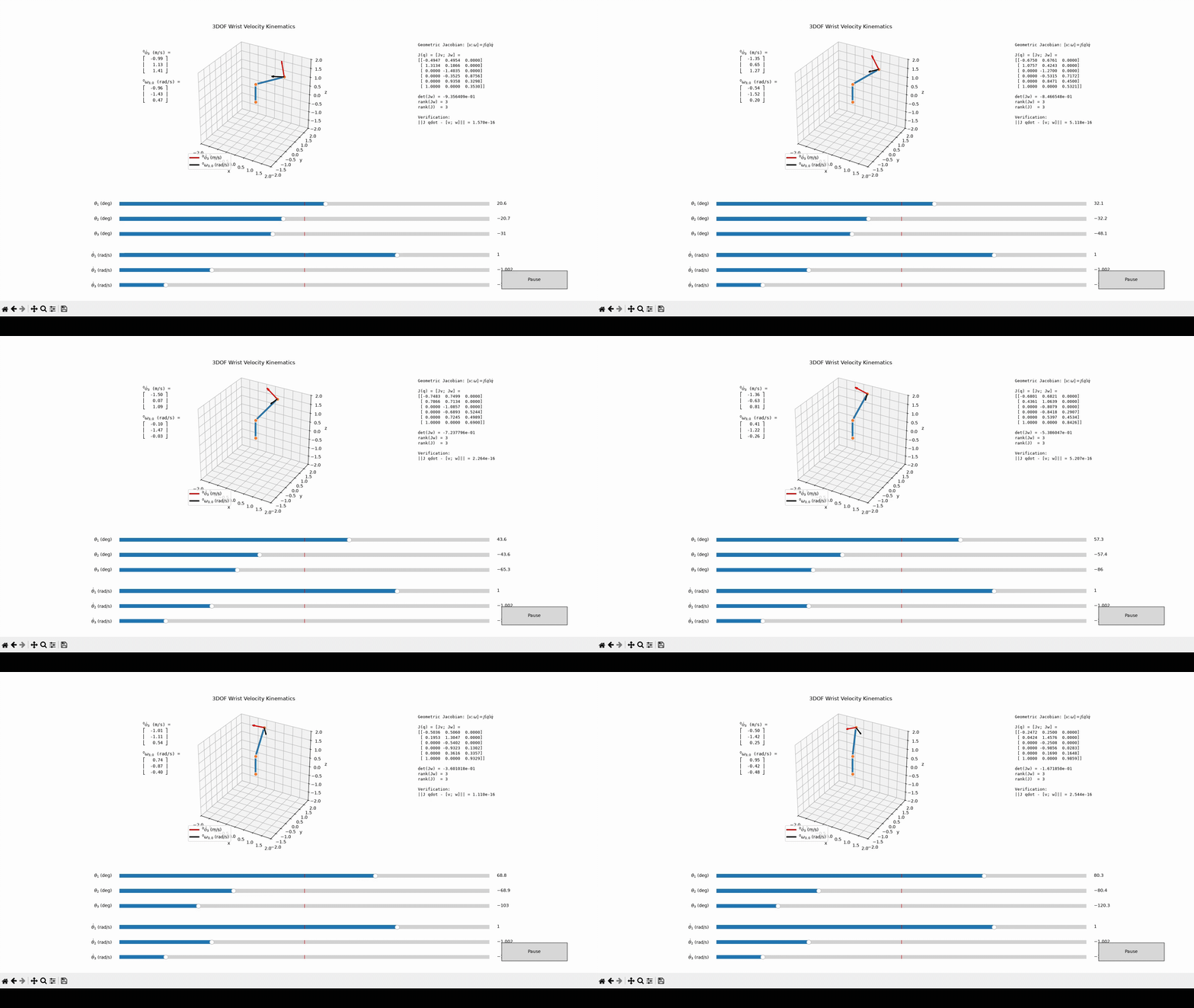
Joint-rate controls compare recursive velocity propagation with the geometric Jacobian velocity map.
Kinematics derivation
The mechanism is a 3-DOF spherical wrist. Now, in order to define the kinematics, we need to define the joint frames. We’ll use the Denavit-Hartenberg convention to define the frames, mainly because that’s just what I learned in school. Typically, a conventional spherical wrist has all frame origins located at the wrist center, with the exception of the end-effector. This removes a lot of complexity, especially as we tackle the Jacobian later on. Something like this:
Figure 1. Conventional spherical-wrist framing.
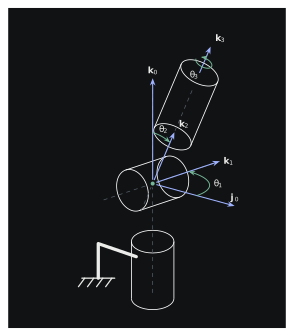
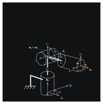
But you know what? That’s too easy. Since the formulas are already known and sitting in my old course textbook, let’s define a new wrist with some impractical frames. It’ll serve as a good test case for our derivations:
Figure 2. Custom wrist framing.
Here we have the base frame at the bottom joint, frames 1 and 2 offset to the ‘center’, and then frame 3 at the end effector. The first thing we need to do is define the DH parameters for this wrist. The table below shows the parameters for each joint:
αi: angle from ki−1 to ki, about ii
di: distance between origins ∼oi−1 and ∼oi, along ki−1
ai: distance between ki−1 and ki, along ii
θi: angle from ii−1 to ii, about ki−1
Link 0 is just the base frame.
DH
θi
di
ai
αi
Link 1
q1
l1
0
−90∘
Link 2
q2−90∘
0
0
−90∘
Link 3
q3
l2
0
0∘
l1 is the distance from the base to the center of the wrist (o0 to o1), and l2 is the distance from the center of the wrist to the end effector (o1 to o3). Now, we can use these parameters to define the transformation matrices for each joint.
For a revolute joint, we have the frame given by the following equations. Here, k× is the skew-matrix of the k vector:
And for a prismatic joint, we have the frame given by:
Ci∼oi=Ci−1Ri,=∼oi−1+Ci−1(δi+dik)
Using the parameters above, we can convert the DH parameters into homogeneous transformation matrices. We will then use these matrices to determine the overall transformation from the base frame to the end-effector frame, giving us the forward kinematics of the wrist.
I’ll be honest because this section was tough to revisit. I actually skipped it and jumped straight to inverse kinematics first. But, it makes the most sense to cover it right after forward kinematics, so here we go.
Angular Velocities
Back to the kinematics. Rather than looking at the whole transformation, including the frame and origin, let’s just look at the frame rotation matrices. These represent the pure orientation changes between frames.
C1=C00C1=C0Q,Q=0C1
Since Q is a rotation matrix, it is orthogonal, so we can write:
QTQ=QQT=I
With a little bit of algebra, we can manipulate this to get:
Q˙=Q˙I=Q˙QTQ
Let’s define Ω=Q˙QT:
Q˙=ΩQ
To verify this property, let’s go back to the orthogonal identity and differentiate it:
QQTQ˙QT+QQ˙T=I,=0
Substituting Ω=Q˙QT yields:
Ω+ΩT=0
or
ΩT=−Ω
Thus, Ω is skew-symmetric. This matrix allows us to extract the physical angular velocity vector. In robotics, the cross-product operator \mathord{\times} converts a 3-element velocity vector into this skew-symmetric matrix form.
Relating this back to those initial formulas, we can express the angular velocity matrix as
0w1,0×=Ω=Q˙QT=0C˙1(0C1)T
Which, in this example, is the angular velocity of frame 1 with respect to frame 0, expressed in frame 0.
To retrieve the actual angular velocity vector, w1,0, we just multiply the angular velocity matrix by the base frame:
w1,0=C00w1,0
Now that we have that, and assuming we’ve calculated the homogeneous transformations, we can move on to calculating the angular velocities of each frame.First, we grab the angular velocities with respect to the previous frame only, expressed in that local frame:
0w1,01w2,12w3,2=θ˙1k,=θ˙2k,=θ˙3k
Remember that each k is the unit z-axis of that respective joint frame about which the rotation occurs.
It is important to remember that angular velocities simply add together, but we need to make sure they are all expressed in the exact same coordinate frame. To make them all relative to and expressed in the base frame 0, we rotate the local vectors forward:
And there we have it, the final angular velocity vectors for our spherical wrist.
Translational velocities
Let’s move on to the translational velocities, or ∼o˙n.
These represent the linear velocities of the origins of each frame with respect to the base frame. We can use the angular velocities we just calculated to find them. While a more direct formula is typically used for the Jacobian, deriving this from first principles helps show exactly what is happening under the hood.
We start by extracting the position vectors of the frame origins from the fourth column of our homogeneous transformation matrices:
Calculating the velocity of each individual frame origin step-by-step down the chain is the first method I learned as it provides a very intuitive approach, so we’ll do the same here. For this, we essentailly track the physical motion outwards, building the velocity profile link by link.
To find how each joint’s rotation we need the radius vectors. Here, we will define each radius as the displacement between the consecutive origins:
We then propagate the velocity outwards from the base. Each link inherits the linear velocity of the previous origin and adds its own rotational cross-product contribution:
As you can imagine, this link-by-link approach, calculating every intermediate step, can get a bit tedious if you only care about the end-effector.
Direct Jacobian Method: each joint’s contribution to the end-effector velocity
Rather than looking at step-by-step segments, let’s instead look directly at how each joint’s rotation impacts the end-effector origin ∼o3 directly.
To do this, we change our perspective on the radius vectors. The radius vector becomes the total lever arm extending from the joint origin in question all the way to that final endpoint:
Using these lever arms, the cross product wi,i−1×0ri gives the linear velocity contribution of each individual joint to the final tip. Summing up the base velocity and the individual joint contributions yields the same total linear velocity of our end-effector origin:
This structural relationship is exactly what lets us build the geometric manipulator Jacobian. The Jacobian maps joint velocities directly to end-effector velocities:
[∼o˙nwn,0]=[J1⋯Jn]q˙=J(q)q˙
By separating out the individual (q˙i) terms from our velocity equations, we reveal the standard column formula for a revolute joint:
Ji=ki−1×(∼on−∼oi−1)ki−1
I know we didn’t really cover it, but for a prismatic joint, there is no angular velocity, only linear velocity along the direction of the joint. So, the Jacobian column for a prismatic joint is simply:
Ji=[ki−10]
Inverse kinematics
Since we went with our own custom wrist frames, the inverse kinematics will need to be derived manually. For a more conventional spherical wrist with all the frames meeting perfectly at the center, the inverse kinematics is well known and can be found in many textbooks. Our inverse kinematics formulas are still quite similar, but let’s go ahead and derive them from scratch.
Our inverse kinematics are still similar, but again, let’s go ahead and derive them.
To start, suppose we know C3 and ∼o3, which represent our target end-effector frame orientation and position. We want to find the corresponding joint angles θ1, θ2, and θ3 to achieve this target. We can begin by looking at our forward-kinematics equations and doing some algebra to isolate the joint angles, keeping in mind the custom frames we defined and tracking which vectors line up.
we post-multiply both sides (multiply on the right) by e−θ3i×. This corresponds to a rotation of −θ3 about the i3 axis and cleanly cancels out that last rotation term.
C3e−θ3i×=eθ1k3×C3=eθ1k0×C0eθ2j×
Now we’re on to something, but we still have too many variables. We need to remove at least one of them. For θ2, the rotation happens entirely about the j axis. If we isolate only the j component of our matrix equation, the θ2 term drops out because a frame rotating around its own j axis leaves that axis unchanged.
e−θ3k3×C3j=eθ1k0×C0j,eθ2j×j=I
By looking at this shared relationship from both the base side and the end-effector side, we can break the main equation into two separate vector conditions.
eθ1k0×j0e−θ3k3×j3=k1,=−k1.
These equations do not bring both vectors onto the exact same target vector. In a conventional wrist they would, but our custom layout changes things. The first equation rotates j0 onto k1, while the second rotates j3 onto −k1. This opposite sign in the second equation comes directly from our DH frame definitions where at θ3=0 we have j3=j2=−k1.
Even though the two target vectors end up with opposite signs, both equations still depend on that exact same intermediate joint-axis direction, k1. From our frame geometry, k1 is perpendicular to both k0 and k3. Therefore, as long as we are in a nonsingular pose, we can calculate k1 directly.
k1=±∥k0×k3∥k0×k3.
The two possible signs give us the two standard Euler-angle branches of the inverse-kinematics solution. We will just carry this ± choice through the math for now and return to what it physically means after we finish solving for the three joint angles.
k1=±∥k0×k3∥k0×k3
Now let’s look closely at how those three frames relate geometrically.
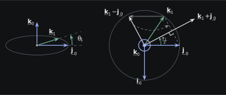
For clarity, we can draw these direction vectors with a common tail even though their coordinate-frame origins do not actually sit at the exact same point in space. This visual shift does not alter our vector math. Since in, jn, and kn are free unit direction vectors expressed in frame 0, their dot products, cross products, sums, and differences remain completely independent of where we choose to sketch them. The physical joint axes themselves still intersect at the wrist center where O1=O2.
eθ1k0×j0=k1
This equation shows that rotating the direction vector j0 about
k0 by θ1 produces k1. It does not mean that
the physical base frame is being rotated. Rather, the rotation operator is being
applied to a copy of the known direction vector j0.
Figure 3. Vector construction for θ₁.
Now we have our constructed triangle with our three vectors. The trick is to translate the vector k1−j0 to form two right triangles:
j0 is known from the base frame, k3 is known from the end-effector frame, and k1 \vect{k}_1 comes directly from our cross-product formula.
To determine the sign of θ1, we need to check whether k1 lies on the positive or negative side of our rotation axis. To do this, recall from figure 3 that positive right-handed rotation about +k0 carries j0 toward −i0. Therefore, a positive θ1 gives k1 a negative i0 component.
sign(θ1)=−sign(k1Ti0)
We can use this exact same triangle trick to solve for θ3, but we have to keep our custom negative sign in mind. At θ3=0, our DH definitions state that j3=j2=−k1. Since frame 3 is built by rotating frame 2 about their common axis k2=k3, we can set up the rotation tracking.
j3=eθ3k3×(−k1),
Or, as we found earlier:
e−θ3k3×j3=−k1
k1, j3, and k3 are all known.
Since k1, j3, and k3 are all known quantities, we can solve the triangle directly.
For the sign, again we are essentially checking whether −k1 lies on the positive or negative side of the rotation axis k3. A positive θ3 rotates −k1 toward i3. Therefore, to determine the sign we check the projection of −k1 onto i3.
Revisiting θ2, we can use a similar approach and the same tricks. But instead of deriving the full the algebraic formula and equivalent vectors, at this point we can just look at it:
And there we have it: θ1, θ2, and θ3 solved for one nonsingular IK branch. There is still one important detail hiding in our first equation for k1: the ± means that there are two possible angle solutions for the same end-effector pose.
We can see where those two solutions come from by going back to the cross product:
k0×k3=cos(θ2)k1
If we take the positive normalized cross product, we are choosing the branch where cos(θ2)>0, or equivalently
−2π<θ2<2π.
This is the branch returned by our Python implementation. Taking the negative direction for k1 gives the other Euler-angle solution, which uses different joint angles but still produces the same end-effector pose. In a more complete solver, we could choose between the two using joint limits, collision checks, or trajectory optimization. That is a bit beyond what we need here though, so we simply use the positive normalized cross product.
Finally, if k0×k3=0, we cannot normalize the cross product at all. This is the wrist’s singular configuration: k1 is no longer uniquely determined, which also means that θ1 and θ3 cannot be recovered individually.
Wrist singularities
Certain configurations create singularities in this wrist, which we can see directly using the Jacobian matrix. A singularity does not mean that the wrist is completely stuck. It means that two Jacobian columns have become linearly dependent, meaning two separate joints are producing the same instantaneous direction of motion. As a result, the wrist temporarily loses one independent degree of freedom (the Jacobian loses rank).
For the angular part of our Jacobian, each column represents one joint axis expressed in the base frame 0.
Jω(q)=[0k00k10k2],0w3,0=Jω(q)q˙.
To see where the determinant comes from, we can write each of those axes in frame 0 coordinates.
For our custom wrist definitions, the final determinant expression works out to:
det(Jω)=−cosθ2.
Therefore, the wrist hits a singularity for the condition:
θ2=±90∘+n180∘,n∈Z.
At these specific configurations, k2 aligns parallel or antiparallel to k0. In other words, joints 1 and 3 are rotating about the exact same physical line in space, meaning their velocity contributions are no longer independent. The Jacobian drops from rank 3 to rank 2. The wrist can still rotate in two independent directions, but it cannot instantaneously produce an angular velocity in every possible direction.
This also explains the failure case in the inverse kinematics derivation. We calculated k1 using k0×k3, but at the singularity, k0 and k3 become parallel, causing that cross product to collapse to zero. The individual values of θ1 and θ3 are no longer unique because only their combined, cumulative effect is defined.
One last interesting note is that near the singularity, although the Jacobian has not quite lost rank, it becomes poorly conditioned. This means that a small requested change in end-effector velocity might demand very large or conflicting joint speeds. In a real-life implementation, these speed spikes may stress the motors and mechanical joints, causing premature wear or failure. And so, these poorly conditioned zones need to be actively avoided just as much as the singularity itself.