2D SCARA Kinematics
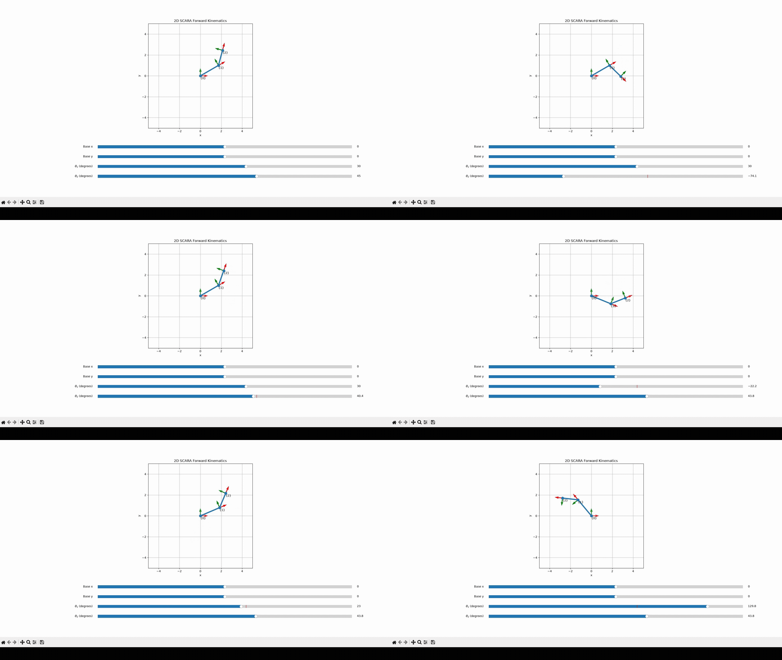
Joint-angle and base-position controls update the arm pose and all three local coordinate frames.
Kinematics derivation
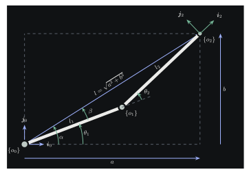
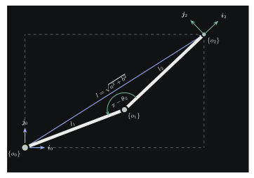
The mechanism is a planar serial chain with two revolute joints. Let the base origin be , and let each link extend along the local -axis of its joint frame. The first link is oriented by relative to the base frame. Because is measured relative to link 1, the absolute orientation of link 2 is .
Forward kinematics
Solving the direct (forward) kinematics of the 2D SCARA is fairly straightforward: given the joint angles, we can determine the location of the gripper in base coordinates.
Now, just looking at the above figure, we can see two things fairly clearly:
And so,
The key thing here is that link 2 () is measured relative to link 1 (). To get link 2’s absolute orientation, and therefore its and components, you need to add and together.
Now, let’s solve the velocity kinematics.
Velocity kinematics
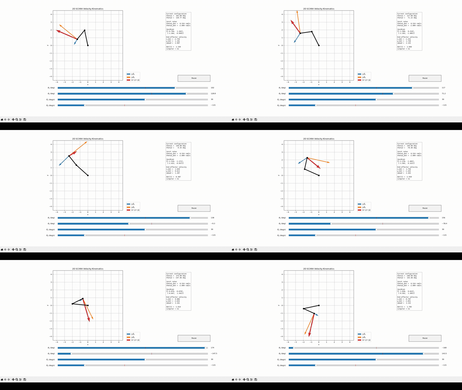
All we really need to do here is take the derivative of the point with respect to time. Using basic differentiation rules and trig derivatives, we take the derivative of the equation above:
Now, rearranging a bit:
This is the Jacobian matrix, which, in this case, is a matrix that maps joint velocities to end-effector velocities in the base frame.
Here, it is easy to see how it represents the end-effector velocities, but it will definitely get messy for higher DOFs!
Inverse kinematics
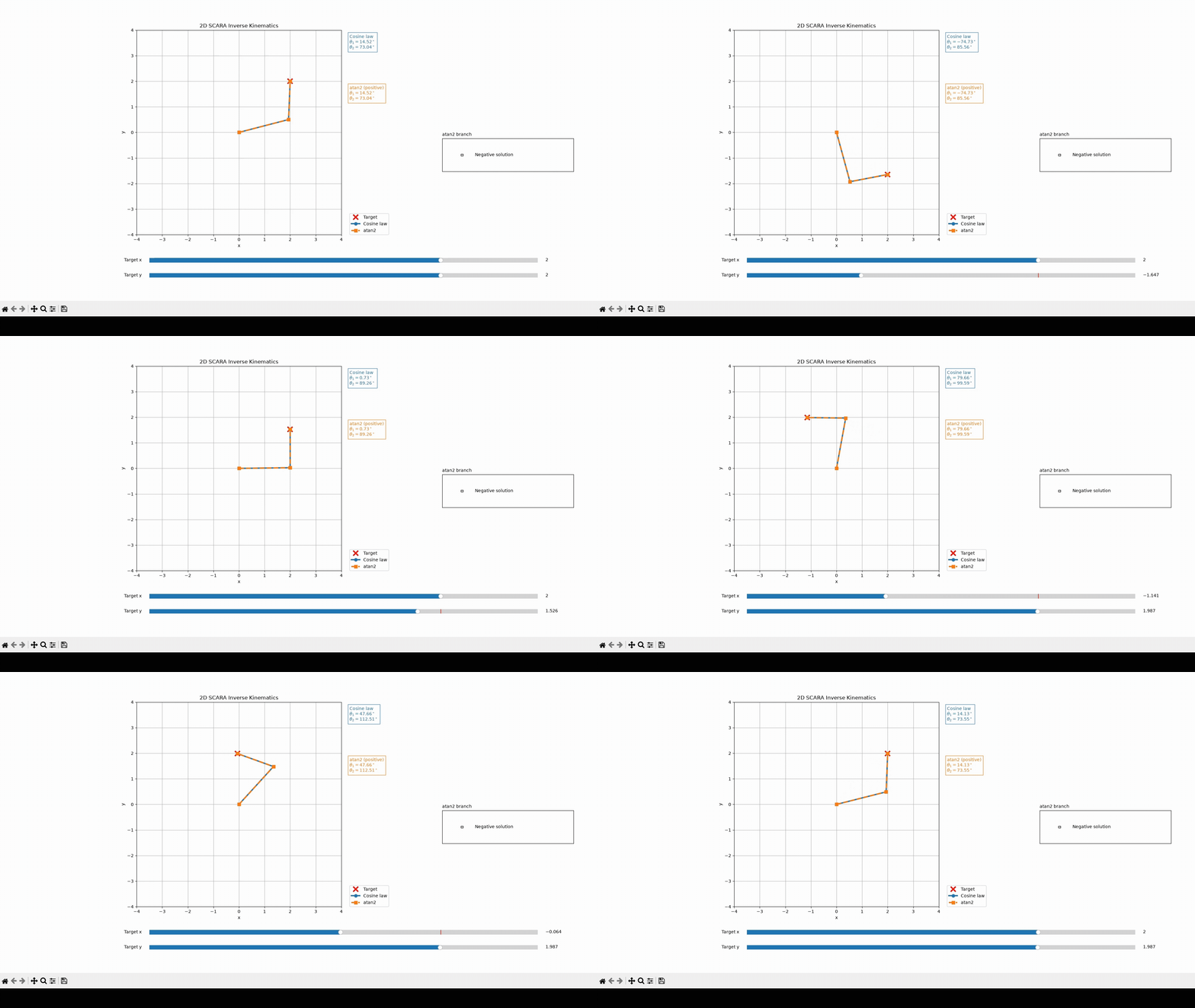
Now for the inverse kinematics, which I find to be a bit more fun. Here, we are given the end-effector position and want to find the corresponding joint angles, and . This is a bit trickier, but we can use the law of cosines to solve for the angles.
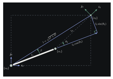
Looking back at the figure, the important part is to draw the hypotenuse formed by and . We can then use cosine and tangent relationships to solve for the various angles. As shown in the figure, we have also labeled and , which are the angles of the drawn triangles. We can solve for these and then use them to determine the joint angles.
First, let’s solve for , since that one is a bit easier. There are technically two ways to do this (well, 1.5, the second way uses the first, but with a few additional steps): a simple method, and a more involved method using atan2 for better accuracy at small angles, as well as the ability to handle quadrants.
The main trick is to solve for this interior angle and recognize that .
So, using the law of cosines, we can solve for :
The equation above works, but we can also use the trig identity to simplify a bit:
And so:
Now, that’s technically all we need. That’s method 1. But to get a little fancy (and improve the accuracy), we can instead use arctangent, or specifically, the quadrant-aware atan2, to retrieve the angle.
Since cosine alone does not distinguish between the positive and negative angle branches, we grab the sine:
Finally, to retrieve the angle while preserving its sign and quadrant, we use:
Moving on to finding .
We can find simply by using the target-origin coordinates:
For , we can also use the law of cosines. For example:
But again, we don’t really like the law of cosines, so let’s use atan2 instead. There is actually another right angle hidden in the figure:
And so:
Here, is already known.
And finally:
There we have it: the inverse kinematics for a 2D SCARA arm. Note that the derivation gives us two possible solutions for , elbow up and elbow down, which also give us two corresponding solutions for .
Repository structure
The derivation above describes the underlying mathematics. In the repository, the calculation layer lives in kinematics.py. It provides 2D rotation matrices along with forward-, inverse-, and velocity-kinematics functions. Three small applications sit above that shared layer:
forward_kinematics.pycontrols the base position and two joint angles while plotting the link geometry and local coordinate frames.inverse_kinematics.pymoves a Cartesian target, compares two analytical formulations, and switches between the positive and negative solution branches.velocity_kinematics.pycontrols joint position and joint rate, displays the Jacobian, and animates the resulting motion.
Keeping the numerical model separate from the interface makes the equations easier to inspect and reuse while each demonstration stays focused on one kinematics question.
Run locally
Create a Python environment with NumPy and Matplotlib, then launch any demonstration independently:
python forward_kinematics.py
python inverse_kinematics.py
python velocity_kinematics.py